Signal Hound VSG60/200 Software Manual

Overview

This document outlines the operation and functionality of the Signal Hound VSG60/200 vector signal generator software. This document will guide you through the setup and operation of the software. You can use this document to learn about the features of the generator and how to access them in the application.

Preparation

System Requirements

Supported operating systems:

• Windows 11/10 (64-bit)
• Ubuntu 22.04/20.04/18.04 (64-bit)

Minimum system requirements:

• Dual core Intel i5/i7/i9 processor, 4th generation or later.
• The software will average less than 1GB of memory.
• USB 3.0 connectivity.

Windows Installation

The latest version of the software can be found on our website at www.signalhound.com.

Once you have downloaded the software, run the installer MSI file and follow the on-screen instructions. You must have administrator privileges to install the software. During installation, the VSG device drivers will be installed.

It is recommended to install the application folder in the default location.

You will need administrator privileges to install the software and drivers.

Driver Installation for Windows

Drivers are distributed by the installer for both 32 and 64-bit systems. After installation the driver files are located at \drivers\x86\ and \drivers\x64\ in the application directory.

If the drivers did not successfully install during the installation process you can manually install them.

The easiest way to install the drivers after the installer has run is to run the Drivers32bit.exe file as administrator. The Drivers32bit.exe file is in the folder at

C:/Program Files/Signal Hound/VSG60

A console will appear to let you know if the installation was successful.

If the drivers still do not install correctly, contact Signal Hound.

Linux Installation

Download the Linux standalone installation directory from the Signal Hound website and follow the included instructions found in the README. All relevant files and drivers are included in the Linux install folder.

Connecting Your Signal Hound VSG

With the software and drivers installed, the VSG can be connected to the PC.

The first time you connect the device to your PC, the PC may take a few seconds to recognize the device and update any drivers. Wait for this process to be completed and the PC to recognize the device before launching the software.

When your device is ready, the front panel LED should emit a solid green color.

VSG60

Plug in the VSG60 using the included USB Y-cable by first connecting the USB 3.0 type A connector to a USB superspeed port on your PC or laptop. Then plug in the thinner USB 2 type A connector (for extra power). Finally, plug in the micro-B connector to the VSG60 until it is fully seated and tighten the thumb screws. Do not overtighten. You should see a solid green LED on the VSG60.

Note: The VSG60 is intended for use only with the included USB cable. Longer cables may result in an intermittent connection, especially around electromagnetic interference.

VSG200

Plug in the VSG200 using the included USB type-C cable. The USB-C connection should be plugged into a port that can negotiate 10W power to adequately power the VSG200. If the unit cannot be powered over USB alone, a power adapter may be used.

Getting Started

Launching the software brings up the user interface (UI). This section describes the UI in detail and how you can use the UI to control your Signal Hound vector signal generator.

Below is a picture of the software after launching.

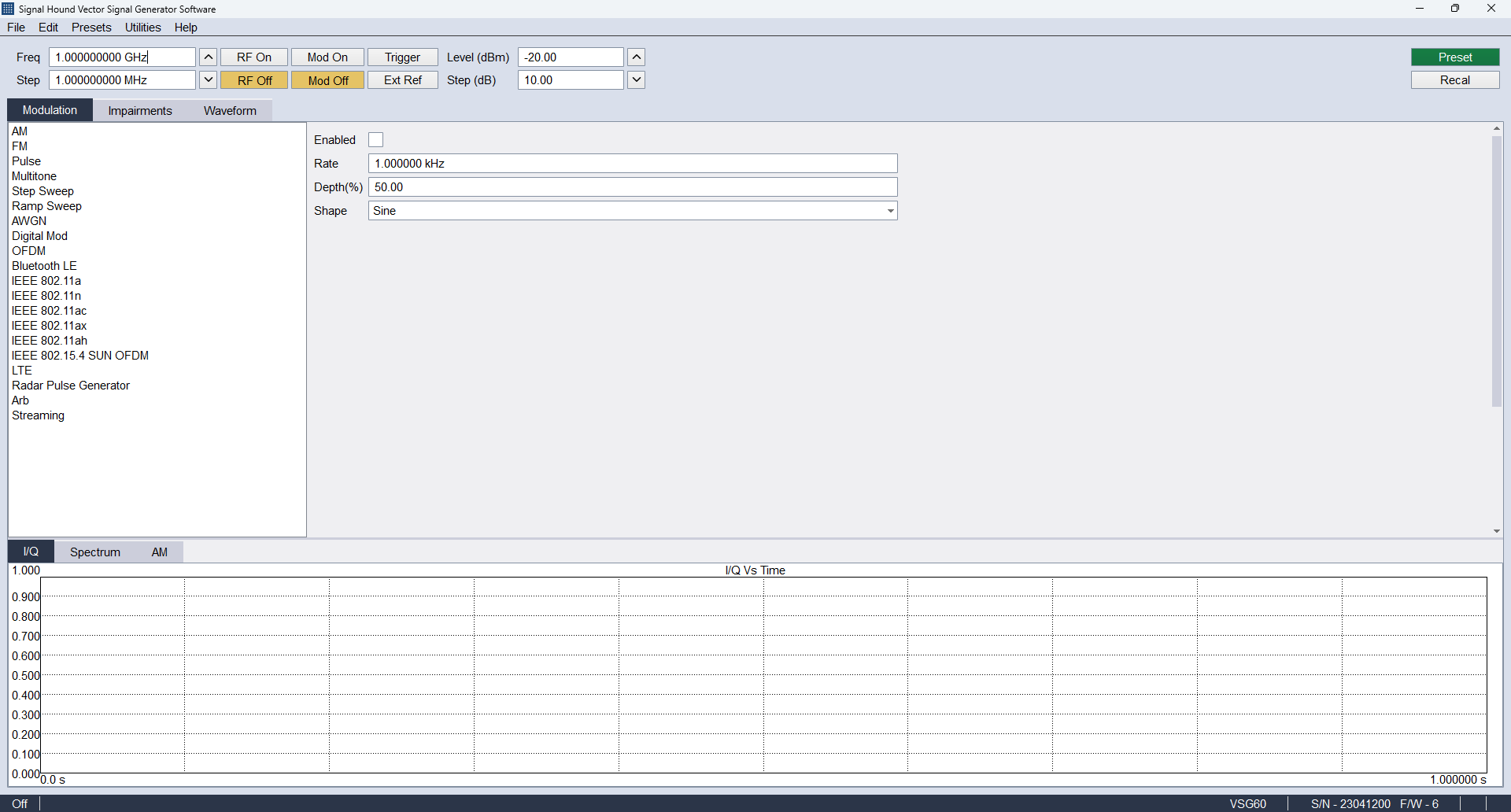
What you will see on program startup.

Menu Bar

The menu bar provides a set of drop-down menus across the top of the application.

Menu Bar

Tab Bar

The tab bar provides controls for switching between our Modulation, Impairments, and Waveform controls.

Tab Bar

Modulation Tab

Select and configure the active modulation type. See the Modulation section for additional details on these controls.

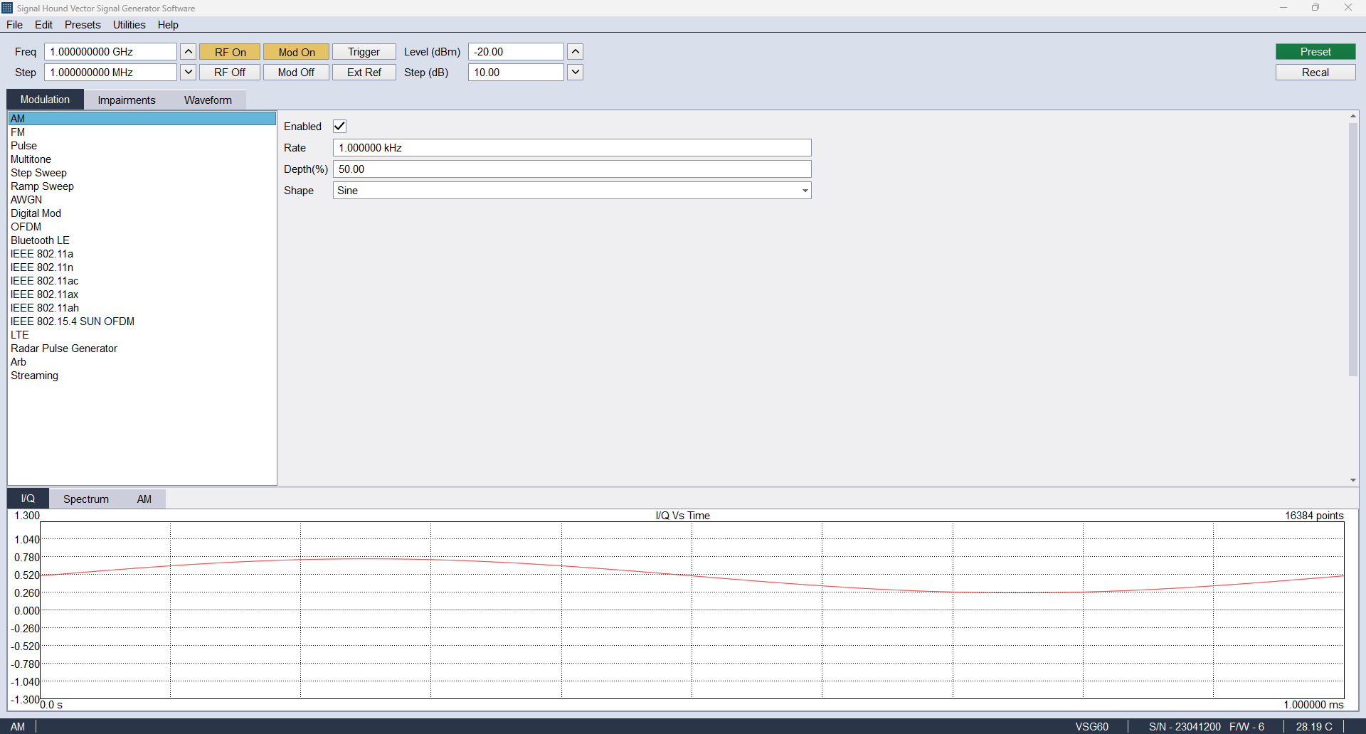
Modulation Tab

Impairments Tab

Used to apply impairments to the output waveform. See the Impairments section for additional details on these controls.

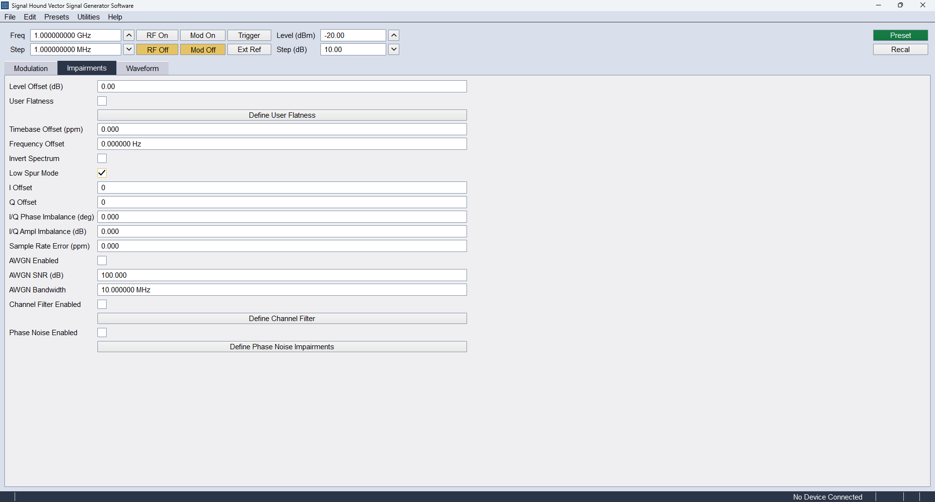
Impairments Tab

Waveform Tab

View metrics on and export the currently configured waveform. See the Waveform section for additional details on these controls.

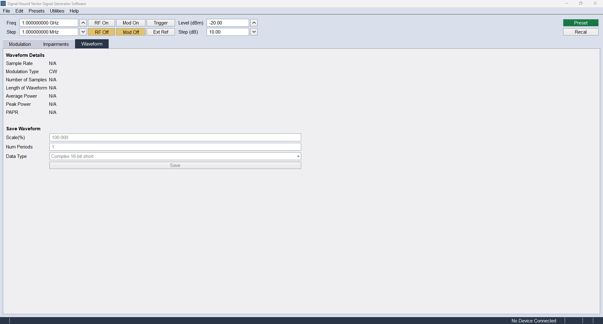
Waveform Tab

Status Bar

The status bar displays information about the device and its current state. In the status bar you will see information about the active device such as model, serial number, and temperature. You will also see the current active modulation.

Status Bar

Menus

File Menu

• Print – Print an image of the application. The image will appear exactly as the software appears to the user.
• Save as Image – Save an image of the application. The image will appear exactly as the software appears to the user.
• Connect – If no device is currently connected, this attempts to establish a connection to a single device. The connect menu shows you a list of all devices connected to the PC. Select one to connect.
• Disconnect Device – If a device is connected, disconnect it and return the software to an idle state.
• Exit – Disconnect the device and close the software.

Edit Menu

• Preferences – Edit several software configuration options.
  • Font Size – Change the font size of the application. Also has the effect of resizing all controls in the application.
  • Accent Color – Change the accent color of the application.
  • Display Waveform Graphs – Show/hide the waveform preview panel.
  • SCPI Enabled – Enable/Disable the ability to control the software via SCPI commands over TCP/IP. When disabled no socket is opened in the software.
  • SCPI Port – Specify the SCPI port used to establish TCP/IP connection for SCPI commands.
  • SCPI Lockout Dialog Enabled – When disabled, the SCPI lockout dialog will not appear when new SCPI commands are sent to the software.
  • Power Saving CPU Mode – See description in software.
  • Image Imbalance Correction – See description in software.

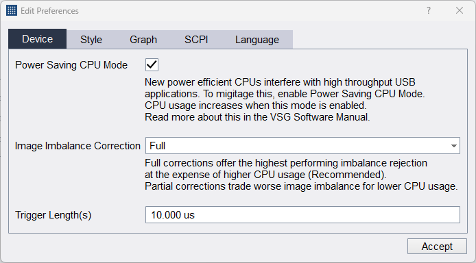
Preferences Dialog

Preset Menu

• Load User Preset – Load a custom user preset file through the file select dialog.
• Save User Preset – Save a custom user preset file through the file select dialog.
• Quick Load – Load from 1 of 9 built in presets.
• Quick Save - Save to 1 of 9 built in presets.
• Save Power On Preset – Save the current configuration as a power on preset. The software only stores one power on preset which is loaded on software startup.
• Delete Power On Preset – Clears the power on preset. After cleared, the software will startup in the default state.

If the power on preset causes issues, such as causing the software to crash on startup making it impossible to delete the power on preset through the software, it can be manually deleted by the user. The power on preset file is located on the PC at

C:\Users\AJ\Documents\SignalHound\vsg60\PowerOnPreset.ini

on Windows PCs. Delete this file and relaunch the application.

Utilities Menu

• Show Error Log – Display the SCPI error log dialog.
• Clear Error Log – Clear the SCPI error log.
• Arb Sequence Editor – Create/Edit .seq files. For a more detailed description see the Arb Sequence Editor section.
• SigMF Editor – Create/Edit SigMF files. For a more detailed description see the SigMF Editor section.

ARB Sequence Editor

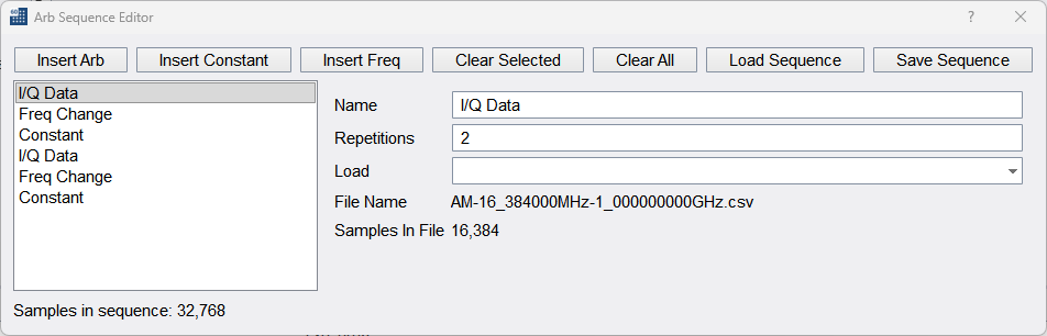
ARB Sequence Editor

ARB sequence files allow customers to define complex frequency hopping signal waveforms. Sequence files have the file suffix (.seq) and are proprietary binary files.

Sequence files are not filtered by the custom channel filter.

The ARB sequence editor is found under the Utilities menu. The sequence editor allows the customer to build sequence files using a convenient GUI. ARB sequence files are user defined ARB files that are constructed of three components,

1. Other ARB files
   1. The files cannot be another sequence file.
   2. The file can be repeated a specific number of times.
   3. Once ARB files are loaded and saved in a sequence, the original ARB files are no longer needed. All I/Q samples in that ARB file are stored in the sequence.
2. Constant values
   1. Customers enter a specific I/Q value to be repeated for a specific number of samples.
3. Frequency switches
   1. Customers specify a new frequency for the VSG to jump to. The frequency change takes 200us to complete.
   2. A sequence does not have to contain any frequency switches. If a sequence contains a frequency switch, there must be at least 2 of them.

Users can add any number of these 3 components to a sequence file and reorder the components in any order.

The maximum number of samples in a fully constructed sequence cannot contain more than the ARB file size limit.

Once all editing is completed, save the waveform. The waveform can now be loaded and transmitted using the ARB output mode.

SigMF Editor

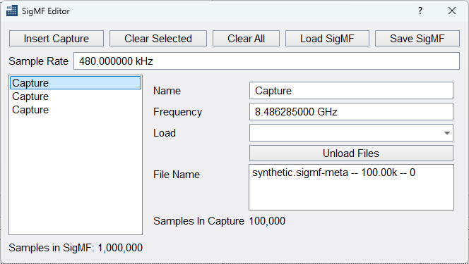
SigMF Editor

SigMF specifies a way to describe sets of recorded digital signal samples with metadata written in JSON. SigMF can be used to describe general information about a collection of samples, the characteristics of the system that generated the samples, features of signals themselves, and the relationship between different recordings.

SigMF Standard is documented at sigmf.org.

The SigMF standard uses .sigmf-meta and .sigmf-data files to define the waveform.

The SigMF editor is found under the Utilities menu. The SigMF editor allows the customer to build SigMF based waveforms using a convenient GUI. SigMF waveforms are defined in the .sigmf-meta file and quadrature binary data that is referenced in the meta data file can be found in the .sigmf-data file.

The SigMF editor requires that you define a Sample Rate for the device and at least 1 Capture. You can define as many Captures as you would like. Each Capture consists of a center frequency and data.

Once all editing is completed, save the waveform. The waveform can now be loaded and transmitted using the ARB controls.

Help Menu

• Software User Manual – Open the user manual in the system default PDF viewer.
• Product Manual – Open the product manual in the system default PDF viewer.
• Signal Hound Website – Open www.signalhound.com in the web browser.
• Support Forums – Open www.signalhound.com/support/forums in the web browser.
• About – Display the software and API version.

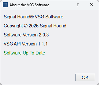
About Dialog

Device Controls

These settings control the device output for all modulation.

• Freq – Specify the output frequency. This will also function as the center frequency for any active modulation. Some modulation types such as step sweep will ignore this frequency.
• Step – Controls the step amount applied when either the frequency arrows or arrow keys are pressed to step the output frequency.
• RF On/Off – Toggles the RF output. When off, the RF output is disabled regardless of other settings.
• Mod On/Off – Toggles the current modulation. When Mod is off and RF is on, a CW is output. When both are enabled, the currently enabled modulation type is output.
• Trigger – Trigger key. In any single trigger generation mode, pressing this button initiates a single trigger event.
• Ext Ref – Specify the timebase source as either internal or external. When Ext Ref is selected, the VSG expects a 10MHz reference signal to be present on the 10MHz reference BNC port.
• Level (dBm) – Specify the output amplitude in dBm.
• Step (dB) – Controls the step amount applied to the output level when either the arrows or arrow keys are pressed.
• Preset – Performs a software reset and loads the software defaults.
• Recal – Regenerates calibration constants for the current environment. The VSG is sensitive to large temperature drift.

Modulation

Modulation Selection

The modulation selection buttons expose the controls for the available modulation outputs. Each button corresponds to a new set of controls to be displayed in the modulation controls area.

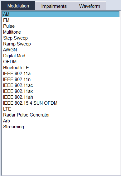
Modulation Selection

Modulation Controls

The modulation controls show related controls for the currently selected modulation. All controls are detailed below.

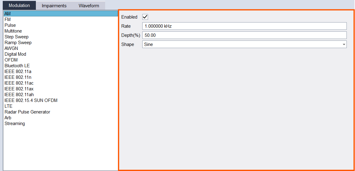
Modulation Controls

AM

• Rate – Specify the AM modulation frequency.
• Depth (%) – Specify the AM modulation depth as a percentage of the output amplitude.
• Shape – Specify the modulation shape of the AM waveform.

FM

• Rate – Specify the FM modulation frequency.
• FM Deviation – Specify the FM modulation deviation. This is the maximum frequency difference between the FM modulated wave and carrier frequency.
• Shape – Specify the modulation shape of the FM waveform.

Pulse

• Trigger Mode – When set to single, a single pulse is emitted for each trigger. A minimum period is still observed equal to or greater than the configured period.
• Width – Specify the time the signal is high during one pulse cycle.
• Period – Specify the time between rising pulse edges.

Radar Pulse Generator

Radar Pulse Generator waveform generation requires a software license. Licenses can be purchased on our website at www.signalhound.com, or by contacting us at sales@signalhound.com.

To manage a purchased license, please see Managing Licenses.

The Radar Pulse Generator mode constructs complex radar pulse trains from pulses, sequences, and off-time. Each pulse can be individually shaped, phase or frequency coded, and repeated with jitter and or a wobbulated repetition interval. A simulated scanning antenna pattern can also be applied.

Sequences are built and edited in the sequence editor, opened from the Radar Pulse Generator mode panel with the New Sequence or Edit Sequence buttons. Sequences are saved to and loaded from .pulseq files.

• Trigger Mode – When set to single, the full waveform (all data) including off period is transmitted on each trigger event. When set to continuous, the sequence repeats continuously.
• Sample Rate – The sample rate at which the generated waveform is transmitted at.
• Enable Antenna Pattern – When enabled, the configured antenna scan pattern is applied to the transmitted sequence.
• Antenna Config – Opens the antenna configuration dialog.
• Antenna Pattern – Displays a summary of the currently configured antenna pattern.
• New Sequence – Opens the sequence editor with a new, empty sequence.
• Edit Sequence – Has the user select sequence (.pulseq) file and opens the sequence editor with that sequence loaded.
• Load Sequence – Load a previously saved sequence (.pulseq) file.
• Loaded Sequence – Displays the name and duration of the currently loaded sequence.

Sequence Editor

The sequence editor lists the pulses, sub-sequences, and off time items that make up the sequence, in transmit order.

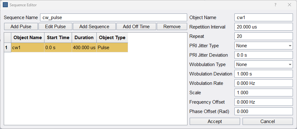
Sequence Editor Dialog

• New Sequence – Discards the current sequence and starts a new, empty one.
• Add Pulse – Opens the pulse editor to define a new pulse and appends it to the sequence.
• Edit Pulse – Opens the pulse editor for the selected pulse.
• Add Sequence – Loads a previously saved .pulseq file and appends it to the sequence.
• Add Off Time – Appends an idle item to the sequence.
• Remove – Removes the selected item from the sequence.

Selecting an item in the sequence table populates the following properties for that item.

• Object Name – The name of the selected pulse, sub-sequence, or off time item.
• Repetition Interval – The pulse repetition interval (PRI): the time from the start of this item to the start of its next repetition.

  Note: For a pulse, this must be long enough to contain its rise time, fall time, and pulse width, including the widest pulse width produced by its pulse width pattern, if configured. For an off time gap, this is the length of the gap.

• Repeat – The number of times this item repeats.
• PRI Jitter Type – The distribuation for the jitter using a Gaussian, Uniform, or UShaped distribution. None disables PRI jitter.
• PRI Jitter Deviation – The magnitude of the PRI jitter.

  Note: For Gaussian jitter the deviation value is 1 sigma. The max value allowed is 3 sigma.

• Wobbulation Type – Periodically varies the repetition interval over time following a Sinusoidal, Saw Tooth, or Triangular pattern. None disables wobbulation.
• Wobulation Deviation – The magnitude of the wobbulation.
• Wobulation Rate – The rate at which the wobbulation pattern repeats.
• Scale – An amplitude scale factor applied to this item, as a fraction of full scale.
• Frequency Offset – A frequency offset applied to this item, relative to the output center frequency.
• Phase Offset (Rad) – A phase offset, in radians, applied to this item.

Pulse Editor

The pulse editor defines the shape, timing, and modulation of a single pulse.

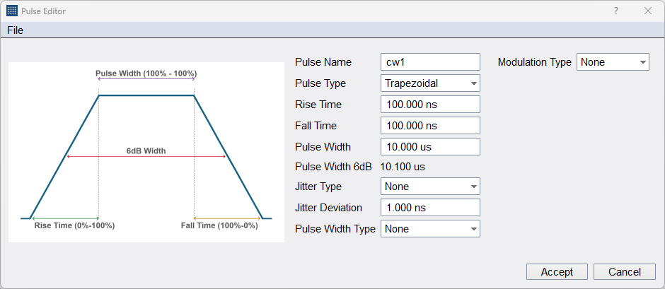
Pulse Editor Dialog

• Pulse Name – The name of the pulse.
• Pulse Type – The shape of the pulse envelope: Trapezoidal or Raised-Cosine.
• Rise Time – The time for the pulse to rise from 0 to full amplitude.
• Fall Time – The time for the pulse to fall from full amplitude to 0.
• Pulse Width – The 100% - 100% pulse width. Hidden when Pulse Width Type is not None, since the width is then governed by the selected pulse width pattern.
• Pulse Width 6dB – The resulting pulse width measured at the -6dB points. Read only.
• Jitter Type – The distribuation for the jitter using a using a Gaussian, Uniform, or UShaped distribution. None disables pulse width jitter.
• Jitter Deviation – The magnitude of the pulse width jitter.

  Note: For Gaussian jitter the deviation value is 1 sigma. The max value allowed is 3 sigma.

• Pulse Width Type – Varies the pulse width across successive occurrences of the pulse, when Repeat is greater than 1 in the sequence editor.
  • None – A fixed pulse width, set by Pulse Width.
  • Linear Ramp – The pulse width ramps linearly between Pulse Width Start and Pulse Width Stop over Number of Pulses, then repeats.
    • Pulse Width Start - Starting pulse width.
    • Pulse Width Stop - Ending pulse width.
    • Number of Pulses - The number of pulses between the starting pulse width and stop pulse width.
  • Staggered – The pulse width cycles through a custom, user-defined list of widths, configured with the Configure Widths button. Widths can be added, removed, or imported/exported as a CSV file from the widths editor.
    • Configure Widths - Opens the Pulse Width Editor for configurating the staggered or completely custom pulse width sequence.
    • Stagger Widths - Label declaring the number of stagger widths that were defined.
  • Stepped – The pulse width starts at Pulse Width Start and increases by Pulse Width Step every Pulses Per Step pulses, for Number of Steps.
    • Pulse Width Start - Starting pulse width.
    • Pulse Width Step - Amount added to each sucessive pulse width.
    • Number of Steps - The number of different pulse widths.
    • Pulses Per Step - The number of pulses for each pulse width step.
• Modulation Type – Applies phase or frequency coding across the pulse.
  • None – No coding is applied. The pulse is a plain CW pulse.
  • FM Chirp – A linear frequency chirp across the pulse, from Start Freq to Stop Freq.
    • Start Freq - Starting frequency, offset from center frequency.
    • Stop Freq - Stopping frequency, offset from center frequency.
  • Barker – A Barker phase code. Code Length selects the code length (2, 3, 4, 5, 7, 11, or 13). Chip Width is computed automatically as the pulse width divided by the order.
    • Code Length - selects the code length (2, 3, 4, 5, 7, 11, or 13).
  • Frank, P1, P2, P3, P4 – Polyphase codes. Order sets the code order. Chip Width is computed automatically as the pulse width divided by the order squared.
    • Order - selects the code length. $$ Order^2 = Number of Chips $$
  • BPSK, QPSK – A custom binary or quaternary phase code. Number of Chips and Chip Width are computed automatically from the custom bit sequence. Use Define Sequence to enter the custom bit sequence in the symbol editor.
    • Define Sequence - Opens Symbol Editor for defining the sequence.
• File
  • Import - Load a saved pulse from a .pul file.
  • Export - Save the currently configured pulse to a .pul file

Pulse Width Editor

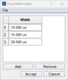
Pulse Width Editor

• Add – Adds an additional pulse width to the table.
• Remove – Deletes the selected pulse width from the table.
• Accept - Accepts the currently configured staggered pulse widths and returns those values to the pulse editor.
• Cancel - Exits the dialog and returns nothing to the pulse editor.
• File
  • Import - Load saved pulse widths from a .csv file.
  • Export - Save the currently configured pulse widths to a .csv file

Antenna Configuration

The antenna configuration dialog simulates a scanning radar antenna. As the simulated antenna scans, its gain at a fixed receiver bearing amplitude-modulates the transmitted sequence over time.

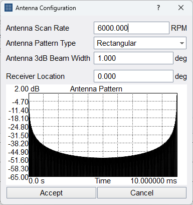
Antenna Configuration Dialog

• Antenna Scan Rate – The rotation rate of the simulated antenna, in RPM.
• Antenna Pattern Type – Rectangular, a flat-top beam of a configurable width, or Custom, an imported gain pattern.
• Antenna 3dB Beam Width – The 3dB beam width of the Rectangular antenna pattern.
• Import Antenna Pattern – Import a CSV file defining a custom antenna gain pattern. Only available when Antenna Pattern Type is Custom.
• Imported Antenna Pattern – The name and number of points of the imported antenna pattern.
• Receiver Location – The simulated bearing, in degrees, of a fixed receiver relative to the antenna's scan.

The antenna pattern plot shows the resulting antenna gain applied to the output over time as the antenna scans past the receiver location.

Multi-Tone

The Multi-Tone mode generates a waveform composed of a table of individual tones, each with its own frequency, power, phase, and enabled state. Click the Initialize button to generate a new tone table with the tone table initialization dialog, then fine-tune individual tones directly in the table below, or import/export the table as a .csv file.

Multi-Tone Modulation Controls

• Sample Rate – The sample rate of the generated waveform. Read only.
• Frequency Resolution – The frequency resolution of the generated waveform. Read only.
• PAPR – Peak to Average Power Ratio for the generated waveform. Read only.
• Initialize – Opens the tone table initialization dialog to generate a new tone table, replacing the table currently in use.
• Add Tone – Appends a single tone to the end of the tone table. The new tone is enabled, with a frequency, power, and phase of 0.
• Delete Tone – Removes the selected tone from the table. If no tone is selected, removes the last tone in the table. If only one tone remains in the table it cannot be deleted.
• Import – Loads the tone table from a .csv file, replacing the table currently in use.
• Export – Saves the current tone table to a .csv file.

The tone table lists every tone that makes up the waveform, one per row:

• Tone – The tone's row number. Read only.
• Enable – When unchecked, this tone is excluded from the generated waveform.
• Frequency – The tone's frequency, offset from the output center frequency. Clamped to ±20MHz.
• Power(dB) – The tone's power in dB relative to the other tones. Clamped to [-100, 100].
• Phase(rad) – The tone's phase, in radians. Clamped to ±360.

Initialize Tone Table

Generates a new tone table, replacing the table currently in use.

Initialize Tone Table Dialog

• Tone Phase – Specify how the phase of each individual tone is generated. The phase selected greatly affects the resulting PAPR of the waveform.
• Seed – Used for seeding the random number generator used when Random tone phase is selected.
• Tone Count – Specify the number of generated output tones. If the count times the frequency spacing would exceed 40MHz, the tone count is reduced to fit, and the frequency spacing is left as specified.
• Freq Spacing – Specify the spacing between each output tone.
• Notch Width – Specify the width of a frequency notch to exclude from the generated tones. Any tone that would fall inside the notch is skipped. A width of 0 disables the notch.
• Notch Center Freq – Specify the center frequency of the notch.

Step Sweep

This mode steps a CW signal across a range of frequencies. Frequency and amplitude are linearly interpolated across the frequency and amplitude ranges. The frequency and amplitude switch time between each output step is 210us. (200us to change frequency and 10us to change amplitude).

• Trigger Mode – When set to single, a full sweep occurs on each trigger.
• Sweep Type – When set to Freq, the application level is used for each output step. When Freq & Ampl is selected, the Start Level and Stop Level are used to create an amplitude ramp across all output steps.
• Start Freq – Specify the start frequency of the stepped sweep signal. When start frequency exceeds stop frequency, the frequency step is negative.
• Stop Freq – Specify the stop frequency of the stepped sweep signal. This is the frequency of the final output step. When stop frequency is less than start frequency, the frequency step is negative.
• Points – Specify the number of output steps. The first step occurs at the start frequency and the final step at the stop frequency.
• Start Level – When the Freq & Ampl sweep type is selected, this is the level of the first step.
• Stop Level – When the Freq & Ampl sweep type is selected, this is the level of the last step.
• Dwell Time – Specify how long the signal dwells at each frequency. A CW is output at each output step.

Ramp Sweep

A CW is swept across a frequency span at a desired output level. The sweep is continuous and thus limited by the instantaneous bandwidth of the transmitter.

• Trigger Mode – When set to single, a full sweep occurs on each trigger. The period is still observed.
• Span – Specify the frequency span of the frequency ramp. Cannot exceed the instantaneous bandwidth of the transmitter.
• Sweep Time – Specify the time it takes the transmitter to sweep through the selected span.
• Period – Specify the time between the beginning of two sweeps. Must be greater than or equal to Sweep Time.

AWGN

In this mode, Gaussian noise is generated over a fixed bandwidth with a fixed channel power.

• Bandwidth – The 3dB bandwidth of the noise signal. This value cannot exceed the instantaneous bandwidth of the transmitter.
• Length – Length of the noise signal buffer. This buffer is cycled through.
• Seed – Used to seed the random number generator. Enables the generation repeatable noise vectors.

Digital Mod

• Trigger Mode – When set to single, the full waveform (all data) including off period is transmitted on each trigger event.
• Samples Off – Specify an off duration after the full waveform is transmitted.
• Symbol Rate - Specify the symbol (chip) rate of the signal. The symbol rate is limited by the device’s maximum sample rate and the oversample amount. For example, the maximum symbol rate with an oversample of 2 is 50MS/s / 2 = 25 MSym/s. The minimum symbol rate is the device’s minimum symbol rate with an oversample of 16 = 12.5kS/s / 16 = 781.25 Sym/s.
• Modulation Type – Specify the modulation type.
• Define Modulation – Define a custom constellation, including differential encoding and offset Q. See custom I/Q modulation editor for more information.
• Filter Type – Specify the pulse shaping filter to be applied to the oversampled waveform.
• Filter Alpha - Specify the filter roll-off factor. Does not apply to custom filters.
• Filter Length – Specify the length in symbols, of the pulse shaping filter. This only applied to non-custom filter selections.
• Define Filter – Specify the pulse shaping filter directly. This filter is applied when custom filter is selected.
• Sequence – Specify the data sequence to be used when generating the waveform. Outputs the full sequence for each trigger.
• Sequence seed – Seeds the random number generator for the PN sequences. Enabled repeatable random number generation.
• Define Sequence – Specify a data sequence to be modulated by bringing up the symbol editor. See the Symbol Editor section.
• FSK Deviation – When FSK is selected, this is the maximum deviation from 0Hz.
• IQ Scaling – Defaults to 1.0. Currently not selectable.
• Oversample – Specify the oversample amount.

Custom I/Q Modulation Editor

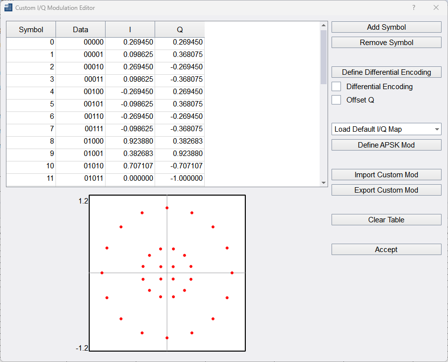
APSK32 in the Custom I/Q Modulation Editor

The Custom I/Q Modulation Editor can be opened with the Define Modulation button on the digital demodulation control panel.

I/Q values can be entered directly in the symbol table. The constellation plot shows the currently entered I/Q values. For loading a large constellation, it is recommended to load a formatted CSV file.

• Add Symbol – Inserts a new symbol row at the end of the symbol table.
• Remove Symbol – Removes the row of the currently selected cell. If no cell is selected, the last row is removed.
• Define Differential Encoding – define the state transitions for differentially encoded modulations
• Differential Encoding – Enables/Disables differential encoding
• Offset Q - Enables/Disables Offset Q
• Load Default I/Q Map – Selects and populates the constellation table with a default selection
• Define APSK Mod – Opens the APSK Editor
• Load – Load a formatted CSV file containing a saved custom constellation.
• Save – Save a formatted CSV file describing the custom constellation.
• Clear Table – Remove all symbols.
• Accept – Verifies the constellation and if the constellation is valid, stores the constellation as the active custom modulation.

APSK Editor

The APSK editor can be opened with the Define APSK Mod button in the Custom I/Q Modulation Editor.

There are four parameters that are used to define each APSK ring. They can each be manually edited in the table found in the APSK editor.

• Ring ID – ID number where 0 is the inner most ring
• **# States** – The number of symbols represented in this ring
• R#/R0 – The ratio of the radius of this ring to the inner most ring(R0)
• Phase – The phase offset of the first state in this ring

Some of the addition controls for the APSK Editor are described below.

• Load Default I/Q Map – Selects and populates the constellation table with a default selection
• Add Row – Adds another ring to the table
• Remove Row – Removes the last ring from the table
• Load – Loads a previously APSK configuration
• Save – Saves the current configuration to a csv
• Accept – Validates that the total number of states is a power of 2, stores the data, and closes the window

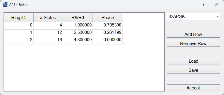
APSK32 in APSK Editor

Custom Filter Editor

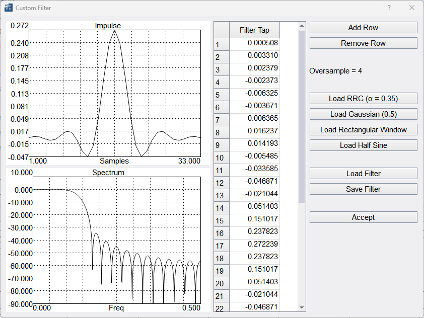
Custom filter editor showing the default RRC filter with alpha 0.35 and oversample 4.

Use the custom filter editor to define your own pulse shaping filter. Easily load default filters for quick modification, or your own custom filters through CSV save/load buttons. Visualize the time and amplitude response of the filter as you edit.

Pulse shaping filters are defined as real, time domain impulses. The filter is applied to the up sampled I/Q data as a complex filter (with the imaginary filter channel equal to zero).

MSK/GMSK Generation

MSK signals can be generated with the software using the proper combination of settings.

MSK is commonly generated in 1 of 2 ways using the Digital Mod output mode.

1. Modulation type of 2FSK with a modulation index of 0.5*.
2. Modulation type of OQPSK with a half-sine filter. The combination of half-sine filter and offset symbols guarantees constant amplitude output.

GMSK is commonly generated using a modulation type of 2FSK with a modulation index of 0.5* and a Gaussian shaping window with 0.5 filter coefficient.

*The modulation index of 0.5 represents the peak frequency deviation over the highest possible frequency component. For a given symbol rate N, the highest possible frequency component is N/2, so a modulation index of 0.5 is half of that, giving you a frequency deviation of N/4.

OFDM

See section OFDM Signal Generation for additional information.

• Trigger Mode – When set to single, the full waveform including idle interval is transmitted on each trigger event. When set to continuous, the waveform including idle interval is transmitted continuously.
• Idle Interval - Specifies a duration after the waveform is output in which the transmitter output is off.
• FFT Size – FFT size used to generate each OFDM symbol. Determines the maximum number of subcarriers.
• Sample Rate – The sample rate at which the generated waveform is transmitted at.
• Guard Band Carriers – Select the number of subcarriers to be used as a guard band.
• Symbol Count – Select the number of OFDM symbols in the waveforms.
• Guard Interval (%) – Specifies the guard interval (GI) of each symbol as a percentage of the FFT Size.
• Null DC – Specify whether the 0Hz subcarrier is nulled out prior to transmission.
• Windowed – If enabled, a raised cosine (RC) window is applied to each symbol.
• Window Length (%) – Length of the RC window as a percentage of the GI.
• Symbol Editor – Press to open the symbol editor. See OFDM Signal Generation section for more information.
• View OFDM Mapping – Shows the OFDM waveform on a symbol vs subcarrier 2D plot, as can be seen in the below image.

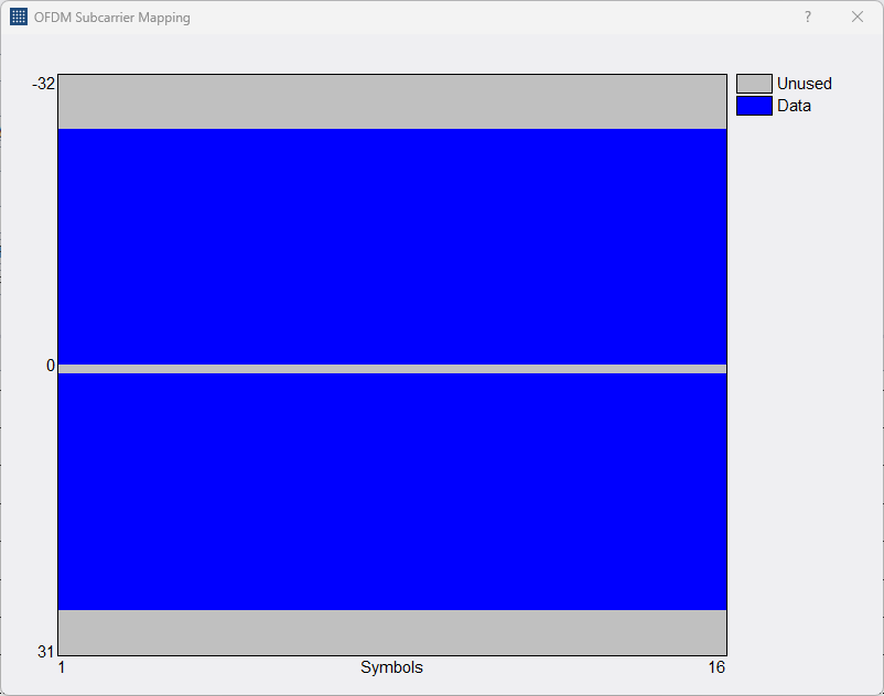
OFDM Mapping

• Save/Load OFDM Configuration – Save and load the full OFDM configuration outside the typical application presets. The configuration can be viewed and edited in other editors if desired.

OFDM Signal Generation

The OFDM signal generation capabilities of the software allow customers to easily define simple OFDM structures for approximating industry standards or developing and testing custom OFDM formats.

OFDM waveforms take the form of a sequence of OFDM symbols where the symbol structure is defined below.

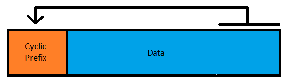
OFDM Symbol

The data section of the OFDM symbol is FFT Size number of complex samples long, and the Cyclic Prefix (CP) length is determined by the Guard Interval (GI). The overall waveform length is,

$$ Waveform Length = Symbol Count * Symbol Length $$

Each symbol is built with the following steps,

1. Initializing all subcarriers to zero.
2. Populating all subcarriers (frequency domain) for that symbol using user provided data in the symbol editor.
3. Nulling out any subcarriers specified in the null DC and guard band subcarriers settings.
4. Performing an inverse FFT.
5. Appending the CP to the front of the symbol.

The symbol editor allows customers to define several resources. Each resource is assigned a symbol range and subcarrier index range. The customer then defines data to populate those subcarriers. Data can be specified directly as I/Q data or generated using a bit stream and constellation mapper.

Subcarriers are populated in order of the resources defined. If two resources contain overlapping subcarriers, the resource lower/later in the list will overwrite subcarriers populated earlier. The symbol editor allows for reordering of resources.

It is for this reason it might be desirable to define certain resources such as pilots after a payload resource. The payload resource might span the usable subcarriers for several symbols, and the appropriate subcarriers can then be overwritten for the pilots. If pilots are ordered before the payload resource, care must be taken to ensure the payload subcarriers do not overwrite the pilots.

OFDM Symbol Editor

Note: Several fields in the symbol editor use a custom range editor to specify ranges of values. To see example inputs to the range editor, right click on the range editor and select Help.

The symbol editor is used to populate the available OFDM subcarriers. Resources are added to the symbol editor using add/remove/copy buttons. Resources can be reordered in the list by dragging them with the mouse. Clicking on a resource shows a list of settings for that resource on the right-hand side of the dialog.

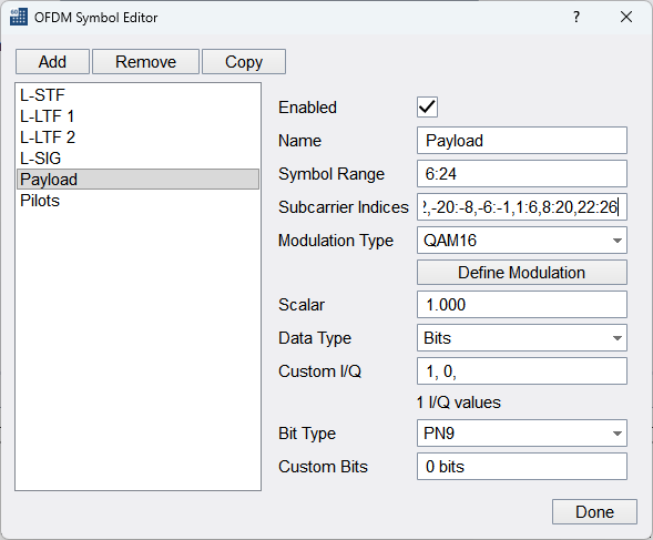
OFDM Symbol Editor

• Enabled – If disabled, this resource is not used to populate the waveform subcarriers.
• Name – Updates the name shown in the resource list.
• Symbol Range – Specify the range of symbols associated to this resource.
• Subcarrier Indices – Specify the symbol indices associated to this resource. The indices are the same for every symbol in this resource. If a different set of subcarriers is needed for a subset of symbols, a new resource should be used.
• Modulation type – Which constellation map should be used when the “Bits” data type is used.
• Define Modulation – Define a custom modulation to be used when “Custom” modulation is selected.
• Scalar – This scalar is applied to all subcarriers associated with this resource.
• Data Type – Specifies how to generate the custom I/Q data for the subcarriers. Bits uses the bit stream and constellation mapper to generate complex data, I/Q Values uses I/Q values specified in the Custom I/Q field.
• Custom I/Q – Specify a custom I/Q sequence. I/Q values are specified as comma separate values of the form, { I1, Q1, I2, Q2, …, In, Qn }. In this example, N I/Q values are specified as 2*N comma separated floating point values.
• Bit Type – Specifies the bit source for the Bits generated complex values.
• Custom Bits – If custom bit source is selected, this user entered source of bits is used.

Bluetooth LE

Use these controls to generate Bluetooth low energy (LE) waveform as specified by the Bluetooth v5.2 specification.

• Trigger Mode – When set to single, the full waveform including idle interval is transmitted on each trigger event.
• Idle Interval - Specifies a duration after the waveform is output in which the transmitter output is off.
• Mode – Specifies the packet format of the waveform. This also controls the sample rate of the generator.
• Channel Index – Specified as a decimal integer. Used for initializing the data whitening. Does not control frequency output. Center frequency must still be controlled manually.
• Samples Per Symbol – Specifies the oversample rate of the generator.
• FSK Modulation Index – Specifies the frequency offset of the FSK modulation. A modulation index of 0.5 (default) specifies a 250kHz frequency offset.
• Gaussian BT – Specifies the Gaussian filter bandwidth time constant. 0.5 is default.
• Filter Length (symbols) – Specifies the Gaussian filter length in symbols. The final filter length is equal to (FilterLengthInSymbols * SamplesPerSymbol) + 1.
• Access Address – Specified as hexadecimal, most significant bit first. (Transmitted LSB first).
• CRC Attached – When enabled attaches 24-bit CRC. CRC is performed over the PDU data prior to whitening.
• CRC Initialization – Initializes the CRC register when CRC is enabled, otherwise ignored.
• Data Whitening – When enabled, whitens the PDU and CRC (if attached).
• PDU Data – Selects the contents for the PDU data section in the packet. Either fill the PDU section with random bits or with a custom payload. No PDU headers are generated by the software. If a PDU header and supporting structure is required, they must be provided using the custom data entry.
• PDU Data Seed – When PN sequences are used for the PDU section, this value is used as the seed. Provided as decimal.
• Bytes – When PN sequences are used for the PDU section, this controls the number of bytes of the PN sequence to transmit. If the PN sequence is shorter than the provided bytes, the PN sequence repeats until the number of bytes is met.
• Custom Data – Specify a custom PDU payload (MSB first). MSB is transmitted first. If the custom data is not a multiple of 8 bits, 0 bits are padded at the end (LSB side).

IEEE 802.11a/n/ac/ax

Note: Transmitting 802.11ax waveforms requires the MATLAB® runtime (free download). Please see the MATLAB® runtime installation instructions.

Note: 802.11ax waveform generation is supported on 64-bit Windows operating systems only.

The software can generate 802.11a/n/ac/ax OFDM waveforms.

802.11ax waveforms are limited to SU waveform types.

Controls for all 802.11 waveforms are described below.

• Trigger Mode – When set to single, the full waveform including idle period is transmitted on each trigger event.
• Idle Interval – Specifies a duration after the waveform is output in which the transmitter output is off.
• Bandwidth Select (ax) – Select between 20 and 40MHz bandwidths.
• Coding Select (ax) – Select coding type. BCC encoding is not available for certain waveform configurations. When those configurations are selected, this control is overridden and LDPC is selected by default.
• Rate Select (a) – Select the modulation and encoding scheme.
• MCS Select (n/ac/ax) – Selects the modulation and code rate for the given standard. Modulation and coding information is displayed in plain text for each MCS selection.
• Guard Interval (n/ac) – Select between long and short cyclic prefix length.
• Guard Interval (ax) – Selects the cyclic prefix length in combination with the LTF duration.
• Sample rate – Controls the device sample rate. Can be used to simulate alternative subcarrier spacings or simulate large sample rate offsets. This setting is coupled to subcarrier spacing.
• Subcarrier Spacing – Coupled to sample rate.
• Oversample Amount – All 802.11 waveforms are fixed to an oversample amount of 1.
• Interleave Bits (a/n/ac) – When enabled the data field symbols are interleaved.
• Scramble Bits (a/n/ac) - When enabled the data field symbols are scrambled.
• Scrambler Initialization – Initializes the data field scrambler.
• Group ID (ac) – Sets the group ID bits in the VHT SIG A1 header.
• Partial AID (ac) – Sets the SU partial AID bits in the VHT SIG A1 header.
• Window Length – When non-zero, a raised cosine window is applied to each symbol using the supplied length in samples. When the guard interval is set to short, the largest window that should be used is 8 samples.
• Data – Select the data source. When “Custom” is selected, the bits configured in the “Custom Data” field is used.
• Bytes – Specify the number of bytes in the data section. Random or custom sequences are cut short if the number of bytes selected is less than the bytes in the sequence. When the number of bytes selected is longer than the selected sequence, bits are repeated until the byte length is met.

IEEE 802.11ah

IEEE 802.11ah waveform generation requires a software license. Licenses can be purchased on our website at www.signalhound.com, or by contacting us at sales@signalhound.com.

To manage a purchased license, please see Managing Licenses.

The software can generate 802.11ah waveforms with the following characteristics,

• 1/2/4/8 MHz bandwidths
• MCS [0-9]
• Short/Long Guard Intervals
• Customizable SIG fields
• Custom payloads/PSDUs
• Adjustable windowing

The following controls are available,

• Trigger Mode – When set to single, the full waveform including idle period is transmitted on each trigger event.
• Idle Interval – Specifies a duration after the waveform is output in which the transmitter output is off.
• Bandwidth Select – Selects between the possible transmission bandwidths
• Preamble – Defaults to short. Not selectable.
• MCS – Modulation coding index. Controls modulation depth and coding + puncturing.
• Guard Interval – Select between short and long. Affects PSDU symbol GI length.
• Interleave Bits – When enabled (default), PSDU bits are interleaved, otherwise, they are not.
• Scramble Bits – When enabled (default), PSDU bit scrambling is enabled. Note: disabling scrambling can lead to long strings of the same bits, which can result in significant PAPR to the point of clipping.
• Scramble Initialization – Seed for the scrambler
• Smoothing Bit – Sets the smoothing bit in the SIG field. Does not perform any smoothing of the waveform.
• Uplink Indicator – Sets the SIG-1 uplink bit field.
• ID – Sets the ID field in the SIG-1.
• Response Indicator – Sets the response indicator field in the SIG.
• Pilots – Set to fixed, not selectable.
• Window Length – Set as a percentage of the PSDU (data) symbol GI length.
• Data Source – Sets the source of the PSDU bits. When set to custom, the bits set in the custom data dialog are used. If any data source is shorter than the target PSDU, the bits are repeated until the desired length is achieved. If the source bits are longer than the PSDU, they are truncated.
• Data Seed - Seed used for PN sequences.
• Aggregation – When enabled, the Len field sets the number of PSDU symbols. Other len is the number of octets in the PSDU.
• Len – See Aggregation.
• Custom Data – Set the bits to be used when custom data source is selected.
• Oversample - When oversample is 2 (default) the waveform is upsampled by 2 before transmitting. This helps with rolloff at the edges. Upsample of 1 may be desired if exporting the waveform.

IEEE 802.15.4 SUN OFDM

802.15.4 SUN OFDM waveform generation requires a software license. Licenses can be purchased on our website at www.signalhound.com, or by contacting us at sales@signalhound.com.

To manage a purchased license, please see Managing Licenses.

The software can generate 802.15.4 SUN OFDM waveforms with the following characteristics,

• Options [1-4] (166.66, 333.33, 666.66, 1333kHz bandwidths)
• MCS [0-6]
• phyOfdmInterleaving 0
• Customizable scrambler seed
• Custom payloads/PSDUs
• Adjustable windowing

The following controls are available,

• Trigger Mode – When set to single, the full waveform including idle period is transmitted on each trigger event.
• Idle Interval – Specifies a duration after the waveform is output in which the transmitter output is off.
• Option – Selects between the possible transmission bandwidths
• MCS Select – Modulation coding index. Controls modulation depth and coding + puncturing.
• phyOfdmInterleaving – Defaults to 0, non-configurable.
• Scramble Seed – Select one of 4 configurable scrambler seeds. Also affects PHR.
• Window Length – Set as a percentage of the PSDU (data) symbol GI length. Performs raised cosine per symbol windowing.
• Data Source – Sets the source of the PSDU bits. When set to custom, the bits set in the custom data dialog are used. If any data source is shorter than the target PSDU, the bits are repeated until the desired length is achieved. If the source bits are longer than the PSDU, they are truncated.
• PN Data Seed - Seed used for PN sequences.
• PSDU Len (octets) – The PSDU length in octets. Also sets the PHR frame length field.
• Custom Data – Set the bits to be used when custom data source is selected.
• Oversample - When oversample is 2 (default) the waveform is up sampled by 2 before transmitting. This helps with roll off at the edges and ensures outer subcarriers are not attenuated. Non-configurable.

LTE

Note: Transmitting LTE waveforms requires the MATLAB® runtime (free download). Please see the MATLAB® runtime installation instructions.

Note: LTE waveform generation is supported on 64-bit Windows operating systems only.

The software provides downlink RMC and test model waveform generation for LTE. The downlink RMC waveforms available are R.0 through R.9 as defined in 3GPP TS 36.101 Annex A.3. The test models available are defined in 3GPP TS 36.141 section 6.3.

By default, the generated waveform is repeated continuously. Pulse or single triggered output is possible using the trigger and idle duration controls.

For downlink RMC waveforms, the following parameters are selectable

• Reference Channel – Select R.0 through R.9
• Cell ID – Physical layer cell ID.
• Duplex Mode – Select between FDD and TDD.
• Subframes – Number of subframes in generated waveform.
• Window length – Specify the OFDM window length in samples.
• Data Source – If the data source is set to custom, the bit sequence specified in the Custom Data dialog is used as the data source. When the number of bits in the specified sequence is shorter than the bits needed to generate the waveform, the sequence is repeated.

For test models, the following parameters are selectable.

• Test Model – Select test model 1.1 through 3.3.
• Bandwidth – Specify the number of resource blocks used.
• Cell ID – Physical layer cell ID.
• Duplex Mode – Select between FDD and TDD.
• Subframes – Number of subframes in generated waveform.
• Window length – Specify the OFDM window length in samples.

ARB

In this mode, a user may load an arbitrary I/Q waveform file to be output by the VSG. Waveforms can be up to 100/200 million samples depending on CPU architecture (x86/x64). Waveforms are loaded completely into system memory and impairments are applied in advance.

In ARB mode, the average power of the waveform is calculated from the I/Q samples and the device gain is adjusted to ensure the average output power of the ARB file is equal to the output level selected.

• Trigger Mode - When set to single, the full waveform (all data) including off period is transmitted on each trigger event.
• Sample Rate – Specify the device sample rate of the waveform.
• Auto Scale – When enabled, the I/Q samples are scaled such that the maximum I or Q value is equal to 1.0. For example, an ARB file containing a single I/Q sample of {1.5, 1.0} would be scaled to {1.0, 0.666}. When disabled, the manual I/Q scale is applied to the waveform.
• I/Q Scale (%) – When Auto Scale is disabled, this scaling factor is applied to every I and Q sample in the waveform. When I/Q scale is equal to 100%, this is equivalent to scaling the waveform to 1 (no scaling).
• Output Signal Average – When enabled, the signal generator output level will be adjusted to ensure the average signal power transmitted is equal to the output level selected. The average signal power is calculated after any I/Q scaling is applied. For example, if the waveform has an average power of -6dBFS (after scaling), and the output level is set to -20dBm, the output level is adjusted to -14dBm to ensure the average signal power output is -20dBm. The output level cannot be adjusted beyond +10dBm. For signals with long off durations, this should be disabled, as the average power of the signal will be significantly lowered with long off periods.
• Period – Specify the period in samples. When period is greater than samples, (period – samples) zeros are output after the waveform.
• Sample Offset – Start offset into the loaded waveform. Using the sample offset and samples to use controls, users can specify only a portion of the ARB file to transmit.
• Samples to Use – The number of samples to transmit starting from the sample offset. Using the sample offset and samples to use controls, users can specify only a portion of the ARB file to transmit.
• Load – Loads an ARB file to be used to generate a custom I/Q signal. See ARB Files for more information regarding the format of these files. If an ARB file is successfully loaded, the characteristics of the signal are displayed in the control area.

Streaming

In this mode, users can load an arbitrary number of binary waveform files for the software to play back in sequence. As opposed to ARB mode, in streaming mode the software reads the waveforms from the files as the VSG is transmitting. This allows for the playback of arbitrarily large waveform files. The files are no longer limited to several hundred million samples, and sequences of billions of samples across several files may be transmitted.

In streaming mode, an I/Q sample magnitude of 1 will equal the output level selected. Unlike ARB mode, the device gain is not adjusted based on the waveform signal average.

• Sample Rate – Specify the device sample rate. The same sample rate must be used for the entire sequence. If different sample rates are desired for different files, it is recommended to resample the binary files prior to loading them into the software.
• I/Q Scale (%) - This scaling factor is applied to every I and Q sample in the waveform. When I/Q scale is equal to 100%, this is equivalent to scaling the waveform to 1 (no scaling).
• Load Files – Load 1 or more files of a given file type. Only files with the given type should be selected. If different file types are desired, load all files of one type first, then select load files again with a different type. Loading additional files will append the new files to the current sequence in the file list.
• Unload Files – Clears all files loaded in the software. If the device is currently streaming, it will be stopped, and no waveform will be transmitted.
• File List – Shows a list of all files loaded into the software. The order of the files from top to bottom is the order in which files are transmitted when streaming is active. User can rearrange files to change the order they are transmitted. If streaming is active when the order is changed, the sequence starts over immediately using the new order. See ARB Files for more information regarding the format of these files.

Because the files are read from disk as they are being transmitted, they should not be renamed/moved/modified while streaming mode is active.

The file list is not saved in the preset files. The file list must be reloaded each time the software is opened.

Disk Speed Requirements for Streaming

Sustained disk read speeds must be fast enough to stream the file continuously. At a 50MS/s sample rate, disk read speeds must be able to sustain 200MB/s for 16-bit complex binary files and 400MB/s for 32-bit complex binary files.

Signal Hound recommends SSD or NVME drives for optimal performance at higher sample rates.

Baseband Waveform Graphs

Plots a preview of the currently configured waveform. For the plots to be populated both RF and modulation must be enabled. Not all waveforms will generate a plot. The baseband data is plotted directly and is only theoretical. The actual output of the signal generator will be subject to the RF impairments of the hardware, such as system noise, phase noise, etc.

There are two plots displayed.

IQ Tab

Graphs the I and Q data vs time of the baseband waveform. The I and Q data are graphed on individual graphs.

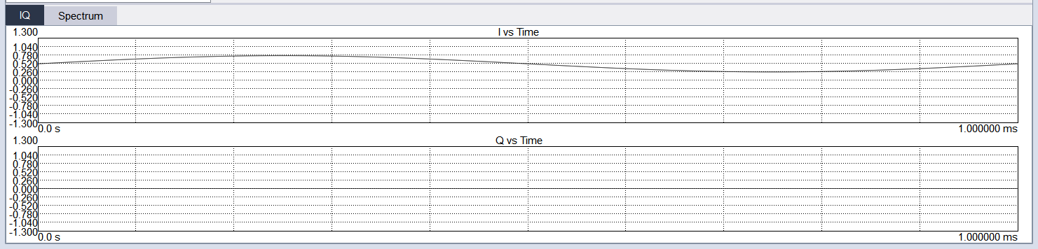
IQ Tab

Spectrum Tab

Graphs the spectrum data of the baseband waveform. This plot is generated with overlapping FFTs on the I/Q data using a max hold detector.

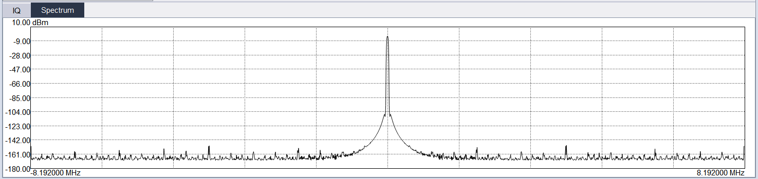
Spectrum Tab

Impairments

• Level Offset (dB) – Specify a power level offset. This offset will be added to the dBm output level of the generator when configuring the transmitter. This offset can be used to compensate for external components such as cables or attenuators. The maximum output level of the transmitter cannot be exceeded with this offset. If the level + offset exceeds the maximum output level of the transmitter, the final output level will be clamped to the maximum.
• User Flatness – When checked, user flatness corrections are applied to the output RF level. This correction will be added to the output level of the generator.
• Define User Flatness – Edit user flatness table. Offsets in the table are linearly interpolated. If the generator frequency is outside the range of the table, the offset applied will simply be outer most point in the table. The offset is a general RF leveling offset and does not apply across the IF bandwidth (baseband) of the transmitter. For baseband flatness corrections, use the channel filter.

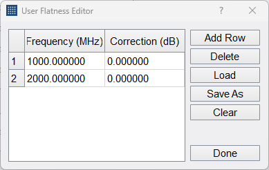
User Flatness Editor

• Timebase Offset – Specify a timebase multiplier in ppm. Available range between [-2,2].
• Frequency Offset – Fixed frequency offset. Applied to the center frequency. Modes that have separate frequency entries such as step sweep mode are not affected by this impairment.
• Invert Spectrum – When enabled, the spectrum is inverted at the devices IF for all output modes. Some output modes such as CW, AM, pulse, and others will not see any effect from this. This inversion is implemented by performing the complex conjugate on all I/Q samples sent to the device.
• Low Spur Mode – When enabled, frac-N spurs are improved through a combination of smart LO choices and digital tuning. The side effect is that the I/Q offset may no longer be at 0Hz.
• I Offset – I channel offset in counts.
• Q Offset – Q channel offset in counts.
• I/Q Phase Imbalance – Specify an I/Q phase imbalance in degrees. The phase imbalance is applied for digital modulation and ARB modes. Any non-zero phase imbalance is split between the real and imaginary channels.
• I/Q Amplitude Imbalance – Specify an I/Q amplitude imbalance in dB. The imbalance is applied for digital modulation and ARB modes. Any non-zero amplitude imbalance is split between the real and imaginary channels.
• Sample Rate Error – Specify a sample rate multiplier in ppm.
• AWGN Enabled – When enabled, gaussian noise is added to the output waveform. Only available in digital mod and ARB modes.
• AWGN SNR (dB) – Specify the desired Signal to Noise ratio (SNR) when AWGN impairments are enabled. Signal power is equal to the average output power of the signal before noise is added. Noise power is the average noise power over the selected AWGN bandwidth.
• AWGN Bandwidth – Specify the AWGN impairment noise width. Cannot exceed 80% of the device sample rate.
• Channel Filter Enabled – When enabled, a user defined channel filter is applied to the waveform. The channel filter can only be applied in digital mod and ARB modes.
• Define Channel Filter - Modify the user defined channel filter.
• Phase Noise Enabled – When enabled, a phase noise impairment is applied to the waveform. See the phase noise impairments section for more information.
• Define Phase Noise Impairments – Modify the user define phase noise impairment.

Phase Noise Impairments

The software can perform real-time phase noise impairments. Using the user defined phase noise curve, a real-time impairment is applied to all waveform types the VSG can generate, including CW outputs. The phase noise will be limited by the performance of the generator itself. A gray phase noise line is shown in the editor which represents the ideal performance of the VSG at 1GHz center frequency. See the product manual for typical plots at different center frequencies.

Phase noise impairments can be defined over the range of 1kHz offset to 2MHz. The impairment is symmetrical around the center frequency. It is recommended to define points spanning the full configurable range.

The phase noise impairment is a real-time impairment and adds additional processing when enabled.

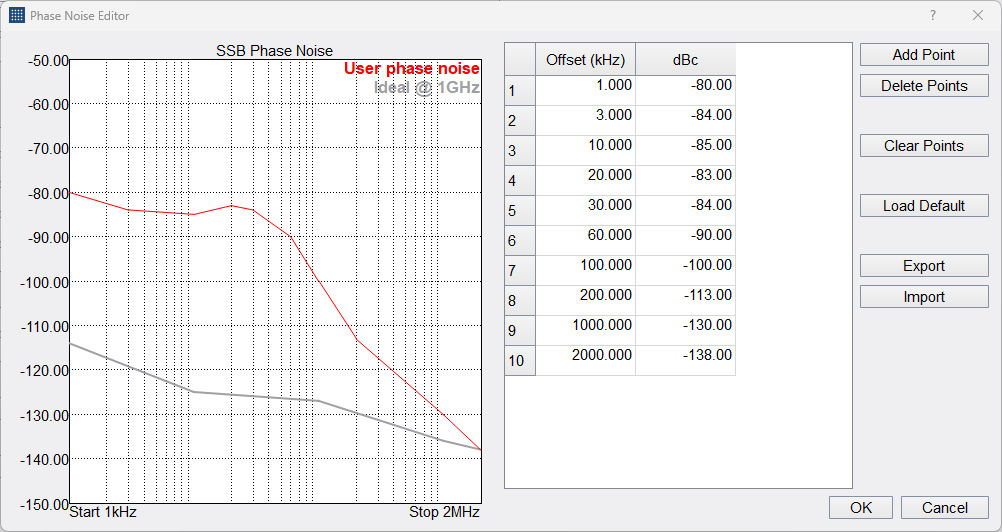
Phase Noise Editor

Channel Filter Editor

Use the channel filter editor to define your own channel response. Easily load default filters for quick modification, or your own custom filters through CSV save/load buttons. Visualize the time and amplitude response of the filter as you edit.

Channel filters are defined as complex time domain impulses. The filter is applied to the waveform as a complex filter.

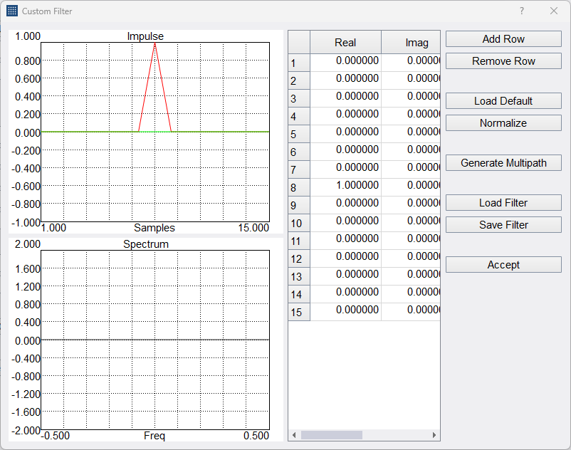
Channel Filter Editor

Generating Multi-Path Channel Responses

Using the “Generate Multipath” button found in the channel filter editor, the software can quickly generate randomized multipath channel scenarios based on basic supplied parameters.

To generate a multipath channel, you must enter the following parameters

• Sample rate – This is the sample rate of the transmitted waveform.
• Delay Spread – The difference in time between the time of arrival of the earliest component of signal and the latest. Typical values are in the hundreds of nanoseconds for indoor scenarios and a few microseconds for outdoor urban environments.
• Filter length – The size of the filter. It should be large enough to accommodate the delay spread.
• Auto seed – When enabled, a random seed is used.
• Manual seed value – Use a manual seed to have reproducible channel filters.

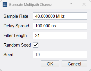
Generate Multipath Editor

Waveform

The waveform tab provides metrics on the currently configured waveform and allows the waveform to be exported to a file.

Waveform Details

Displays data about the currently configured waveform.

• Sample Rate - The device sample rate for this waveform
• Modulation Type – The type of modulation enabled in the Modulation controls
• Number of Samples - The number of samples to be saved
• Length of Waveform – The length of the waveform in time. This is calculated by multiplying Sample Rate and Number of Samples.
• Average Power – Average Power for the waveform
• Peak Power – Peak Power for the waveform
• PAPR – Peak to Average Power Ratio for the waveform

Save Waveform

Controls for exporting the currently configured waveform to disk.

• Num Periods – The number of times to repeat the waveform when saving.
• Data Type – Data type for the output file. The supported options are Complex 16-bit shorts and Complex 32-bit floats. This type will be applied to the output appropriately based on the selected extension.
• Save –Save the configured waveform. You will be able to select the extension. Choices include CSV, Binary, or SigMF as the output file type. A default name is selected based on the current configuration.

External Triggering

The VSG has a 3.3V logic trigger output that can be used to synchronize external devices to the RF output of the VSG. The external trigger is used in several output modes, including ...

• Pulse output
• Ramp sweep
• All digital modulations
• ARB output

In these output modes, the external trigger is driven high at the beginning of the RF waveform in both single and continuous operation. The output is driven high for 10us (default).

In single operation, 1 external trigger is transmitted for each trigger event (pressing the trigger button or triggering via SCPI).

In continuous operation, the trigger operates at a maximum rate of 2kHz. Signals shorter than 500us will be transmitted 2 or more times to ensure the trigger frequency is less than or equal to 2kHz. For example, a 400us signal will be transmitted twice for every external trigger. A 20us waveform will be transmitted 25 times for every external trigger.

Symbol Editor

The symbol editor is a dialog window used to create custom data sequences in the software for the various digital modulations. The symbol editor makes it fast and easy to enter custom binary sequences. The symbol editor allows you to save sequences and load them for later use.

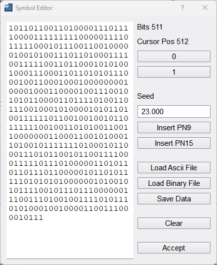
Symbol Editor

The symbol editor consists of the current binary output on the left and several action buttons on the right. Above the binary output, you can see the current size of the binary sequence measured in bits and the current bit position of the cursor. Using the buttons on the right of the output sequence, you can add additional bits into the sequence at the cursor location. You can also insert pseudo-noise sequences with the Insert PN9 and Insert PN15 buttons. You can manually set the seed for the pseudo random sequences for repeatability tests.

Using the Load File and Save Data buttons you can export and import text files containing binary sequences. Files are saved in an ascii binary (‘0’ or ‘1’) format. Ascii files can be loaded as either ascii binary or hex.

Loading an Ascii File

When ascii files are loaded they are interpreted as either ascii binary or hex. If all characters read are ‘0’ and ‘1’, the file is interpreted as ascii binary. If any character is ‘2’ through ‘F’, the whole file is interpreted as ascii hex. If any character falls outside the hex ascii range, the file will not be loaded.

Interpreting the Binary Sequence

The binary sequence will be interpreted differently depending on modulation type selected. The sequence will be split according to how many bits per symbol are required for the selected modulation. The sequence is zero-padded at the end of the sequence if needed to create a sequence of an integer number of symbols.

ARB Files

The software allows you to load custom I/Q ARB files which fully define the device output. The files follow a standard format which is described below.

CSV Files

These files should have a .txt or .csv extension. They should be in plain text. Each line should contain a pair of complex values (I/Q) separated by a comma. Each line should end in a newline. The file is read until a line no longer follows this format.

I(0), Q(0),
I(1), Q(1),
…
I(n), Q(n)

Binary Files

The software can load binary files with extension .bin .dat and .iq. These files should be interleaved complex values, either 16-bit integer or 32-bit floating point scaled to 1.0 magnitude.

Midas Blue

The file extension for these files should be .tmp or .prm. Only files that have these characteristics can be loaded properly,

• Little endian headers and data
• Cannot be detached
• Must be 1D complex data (type code 1000)
• Must have data_format of ‘F’, ‘D’, or ‘I’

Sample rate is retrieved from VariableHeader.x_delta.

WAV Files

The software can read I/Q data stored in WAV files with the following format.

• Must be a 2-channel file
• I-values are stored in channel 1, Q-values are stored in channel 2
• Must have either WAVE_FORMAT_PCM or WAVE_FORMAT_IEEE_FLOAT audio types.
• Supports 16-bit shorts and 32-bit floats only.

Arb Sequence files

ARB sequence files allow customers to define complex frequency hopping signal waveforms.

ARB sequence files are generated using the sequence editor in the Utilities menu. See ARB Sequence Editor for more information.

SigMF files

SigMF files allow customers to define complex frequency hopping signal waveforms.

SigMF files are generated using the SigMF editor in the Utilities menu. See SigMF Editor for more information.

Example: Creating a Frequency Hopping Sequence File

This section illustrates creating a simple frequency hopping sequence using the ARB sequence editor. This example uses an ARB file found in the example ARB files which can be downloaded using the following link https://signalhound.com/support/product-downloads/vsg60a-downloads/ Customers may substitute their own ARB file if desired. The sequence file that is generated from this example also is present in the ARB file download.

First, open the ARB sequence editor from the Utilities menu. You should see an empty sequence editor.

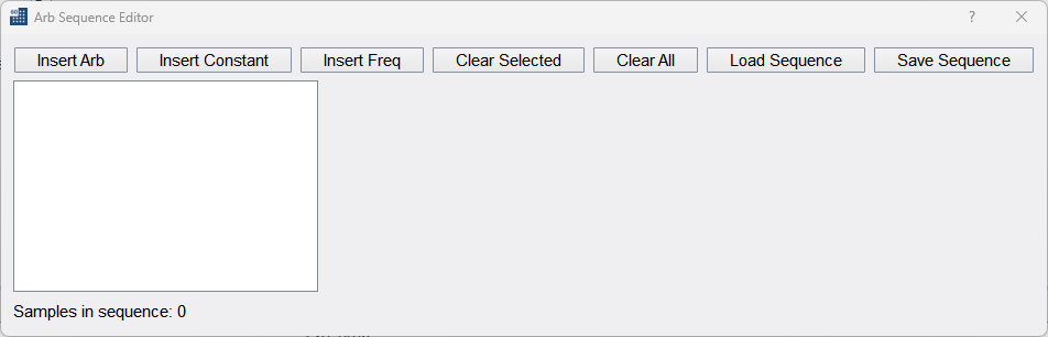
Empty Arb Sequence Editor

Insert the following components and configure each component as follows.

1. Insert Freq Change
   • Set frequency to 990MHz.
2. Insert ARB
   • Load the WLAN80211a.csv waveform and set repetitions to 2.
3. Insert Constant
   • Set I and Q values to zero and set sample count to 1000.
4. Insert Freq
   • Set frequency to 1010MHz.
5. Insert ARB
   • Load the WLAN80211a.csv waveform and set repetitions to 1.
6. Insert Constant
   • Set I to 1 and Q to 0 and set sample count to 2000.

You should now see the following in the editor.

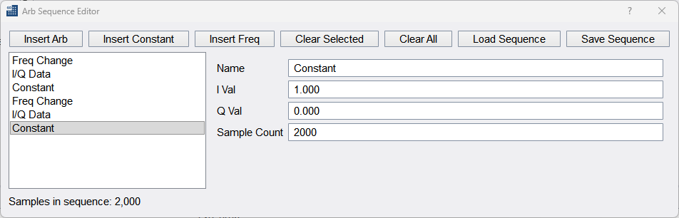
Sequence editor after inserting 6 components.

Now save the sequence file as “user_seq_example.seq” and close the sequence editor. Navigate to the ARB output mode and load a custom sequence file and select our sequence example file. Configure the sample rate to 40MHz. Disable output signal average. When finished the UI will look like this.

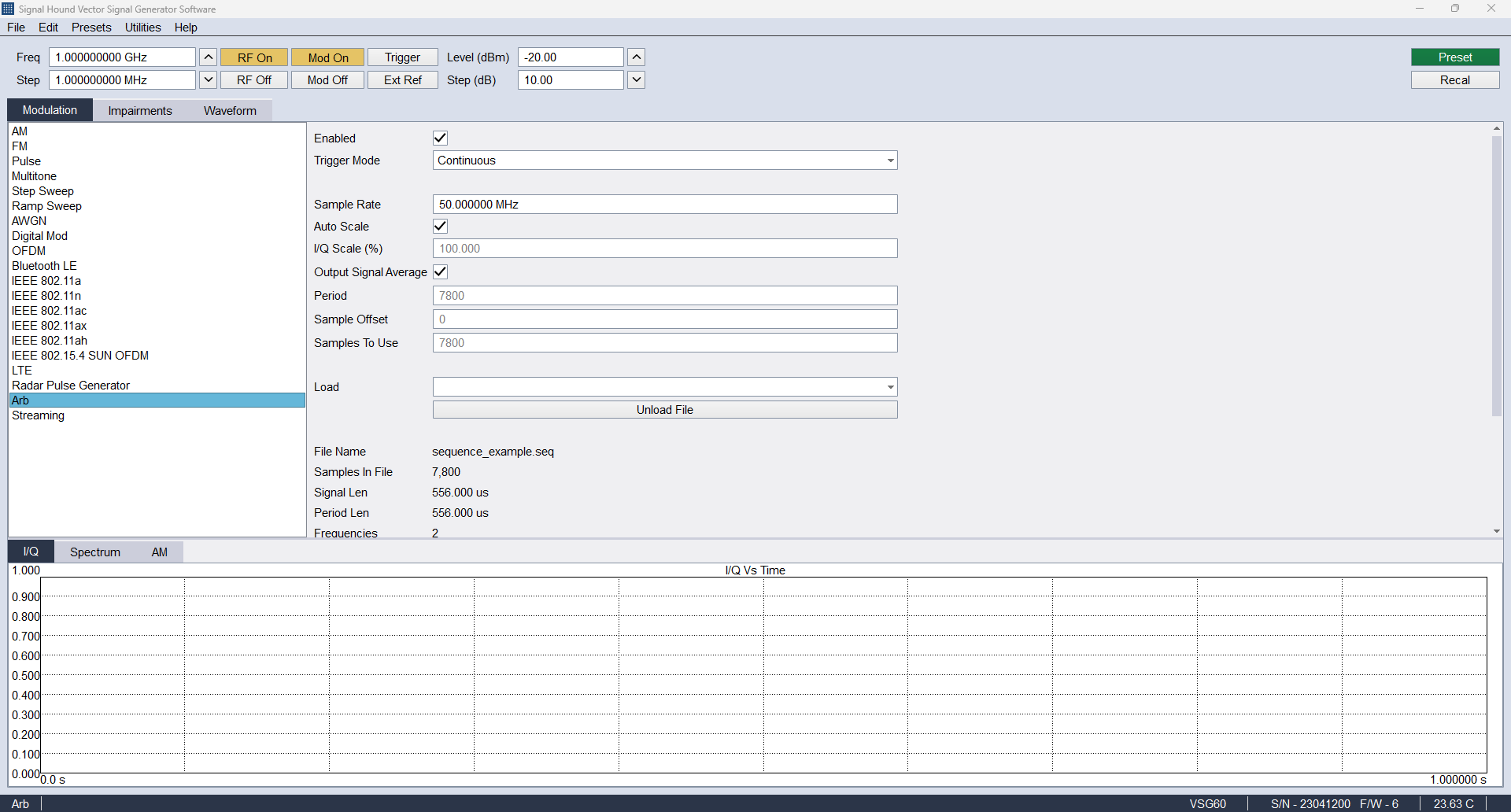
UI with custom sequence loaded.

With the sequence loaded and RF/Mod enabled, the following sequence is transmitted.

• The generator will switch to 990MHz center frequency, in 200us.
• The generator will output the ARB file twice, a total of 3200 samples over 80us.
• The generator will output no signal for 1000 samples, or 25us.
• The generator will switch to 1010MHz center frequency over 200us.
• The generator will output the ARB file once, a total of 1600 samples over 40us.
• The generator will output a CW signal for 2000 samples, or 50us.

Using the SM200 spectrum analyzer we can see this sequence in the picture below. The upper left plot shows the leading frequency change. The waterfall plot is read top-down. The output at 990 on the left side of the waterfall is transmitted first, followed by the output at 1010 on the right later.

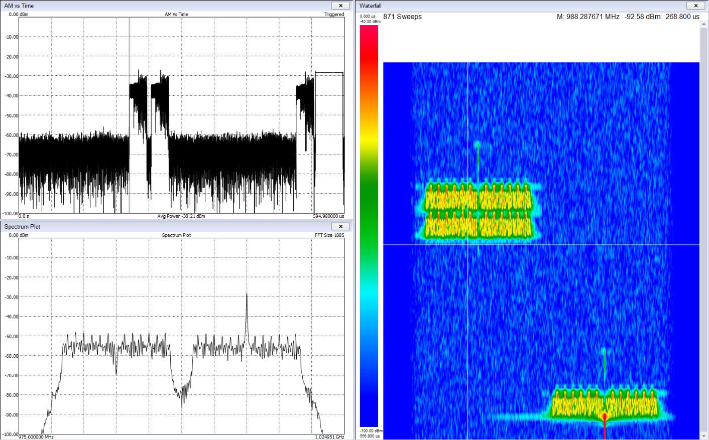
Custom sequence shown on spectrum analyzer.

Managing Licenses

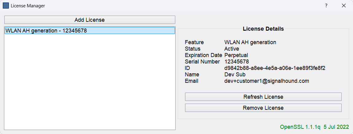
License manager dialog

The license manager dialog is used to add, activate, remove, and see details about licenses stored on the machine. The license manager can be accessed through the utilities menu in the VSG software.

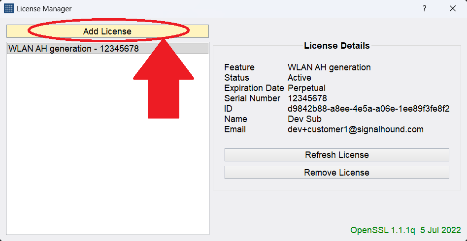
All licenses in use locally are displayed in the list on the left, with their associated serial number. Expired licenses are shown in red text. Clicking on a license will show its details on the right. It will also enable actions to be performed on it with buttons on the right.

To enable a licensed feature, an active license must be added to the local store. Instructions on how to do this are below.

Adding and Activating a License

After purchasing a Signal Hound software license, you will receive a license key that is used to activate the license in the VSG software. An internet connection is needed for activation, but from then on, the license is stored locally, and no internet connection is needed.

1. First, make sure the VSG software is up to date. You can download the latest version from ://signalhound.com.

2. Navigate to your account page on the Signal Hound website.
   

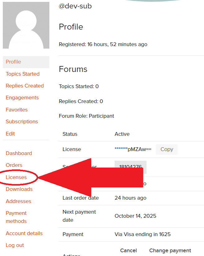
3. Click “Licenses” in the sidebar.
   

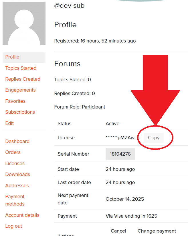
4. Click the “Copy” button to copy the license key to your clipboard.
   

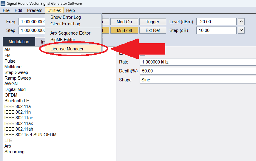
5. In the VSG software, open the License Manager from the Utilities menu.
   

6. In the License Manager utility, click the “Add License” button.
   

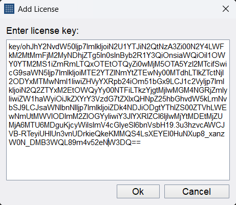
7. Paste the license key into the text field and click “Ok”.
   

8. When prompted, enter the serial number of the Signal Hound spectrum analyzer you would like to associate with this license. When the license becomes associated with a spectrum analyzer via its serial number it is considered active.

Removing a License

To remove a license, select it from the list, and press the Remove License button. This only removes the license information from the local machine, but does not affect the license itself, which can be re-added on this or another machine.

Refreshing a License

If a license was renewed or otherwise altered, the local information can be updated to reflect these changes by pressing the Refresh License button.

Troubleshooting

The Device Does Not Connect to the Software

• Confirm the USB 3.0 cable is connected the VSG to the PC and is solidly connected at both ends.
• The USB cable must be connected to USB 3.0 ports on the PC. USB 3.0 ports are usually blue or are labeled with an “SS” marking near the port. If you are unsure if your PC has USB 3.0 ports, refer to your PC manual or contact Signal Hound.
• Once the USB cable is connected, ensure the LED on the device is solid green.
• If you use a USB 3.0 hub, try removing the hub and connecting the device directly to the PC.
• Manually reinstall the USB 3.0 driver. Navigate to the driver directory at C:\Program Files\Signal Hound\VSG60\drivers\x64. Find the cyusb3.inf file, right click this file and select “Install”. Once installed successfully, power cycle the device and attempt to reconnect the device.
• Try a different USB 3.0 cable. You can use any single ended USB 3.0 cable for this test. You can often find compatible cables on USB 3.0 hard drives. If you do not have a spare, you can request one from Signal Hound.
• Verify the PC meets the system requirements (listed near the top of this document). In particular, the CPU requirement.
• Try a different PC.

If the device works on a different PC, contact Signal Hound with information about the non-working PC for additional troubleshooting help. If the device does not connect on multiple PCs, contact Signal Hound.

The Device Does Not Transmit a Stable Signal

If the output of the device does not seem continuous or stable, try the troubleshooting steps below.

This issue will appear as a pulsed output on a continuous signal like a CW or a continuously modulated signal like AM/FM. This behavior can be observed in the time domain or frequency domain with a spectrum analyzer. This indicates the PC is unable to meet the CPU or USB streaming requirements to sustain the data rates required for the given configuration.

• Verify the PC meets the system requirements (listed near the top of this document). In particular, the CPU requirement.
• Our software is optimized for Intel processors. If using an AMD processor, this could be the reason. Please contact Signal Hound with information about your PC in this event.
• Enable the high-performance power plan. (See picture below) If high-performance is not available, “show additional plans” can be expanded to reveal more plans. Some low power laptops might not have a high-performance plan.

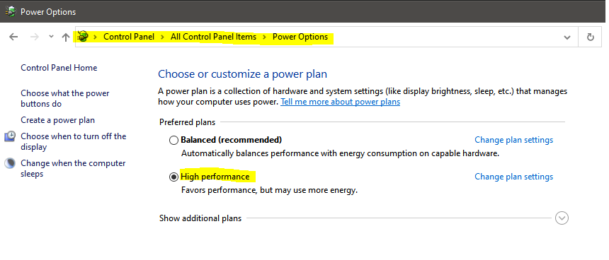
Enable high performance power plan

• If using a USB 3.0 hub, remove the hub and connect the device directly to the PC.
• Try connecting the USB 3.0 cable to different USB 3.0 ports on the PC. If using a desktop, avoid front panel USB 3.0 ports. Instead connect to ports on the rear of the PC.
• If any other USB devices are connected or are being actively used (such as a Signal Hound spectrum analyzer) disconnect that device and run the VSG by itself.
• If any other high CPU usage software is being run simultaneously, close that software and run the VSG by itself.
• If any anti-virus or corporate security software is installed on the PC, temporarily disable it before running the software.
• Try running the device with and without the “Power Saving CPU Mode” checkbox enabled in the Preferences menu in the software.
• Try using a different USB 3.0 cable. You can use any single ended USB 3.0 cable for this test. You can often find compatible cables on USB 3.0 hard drives. If you do not have a spare, you can request one from Signal Hound.
• Disable C-states in the BIOS. Newer Intel processors have low power sleep states that can interfere with USB transfers causing enough latency to interrupt the RF output. Disabling C-states in the BIOS will eliminate this at the expense of higher power usage on the machine. Even if this is not a tradeoff you are willing to make, it is helpful to determine if this is the source of the issue. If it is and you cannot afford disabling this permanently, this PC may not be usable with the VSG.

Using Multiple USB 3.0 Devices on Linux

There are system limitations when attempting to use multiple Signal Hound USB 3.0 devices* simultaneously on Linux operating systems. The default amount of memory allocated for USB transfers on Linux is 16MB. A single Signal Hound USB 3.0 device will stay within this allocation size, but two devices will exceed this limitation and can cause connection issues or will cause the software to crash.

The USB memory allocation size can be changed by writing to the file

/sys/module/usbcore/parameters/usbfs_memory_mb

A good value would be N * 16 where N is the number of devices you plan on interfacing simultaneously. One way to write to this file is with the command

sudo sh -c ‘echo 32 > /sys/module/usbcore/parameters/usbfs_memory_mb’

where 32 can be replaced with any value you wish. You may need to restart the system for this change to take effect.

*Includes both Signal Hound USB 3.0 spectrum analyzers and signal generators.

Calibration and Adjustment

For more information regarding calibration and adjustment see the product manual on our website or shipped with our software or contact Signal Hound.

Warranty and Disclaimer

©2026 Signal Hound. All rights reserved.

Reproduction, adaptation, or translation without prior written permission is prohibited, except as allowed under the copyright laws.

The information contained in this manual is subject to change without notice. Signal Hound makes no warranty of any kind regarding this material, including, but not limited to, the implied warranties or merchantability and fitness for a particular purpose.

Signal Hound shall not be liable for errors contained herein or for incidental or consequential damages in connection with the furnishing, performance, or use of this material.

Refer to the End User License Agreement for additional warranty and disclaimer information covering the VSG software.

Credit Notice

Windows® and Excel® are registered trademarks of Microsoft Corporation in the United States and other countries.

Appendix

Command Line Options

The following command line options are available when launching the software.

--hidden, Hides the user interface, including on the taskbar. To be used in conjunction with SCPI to allow for ‘headless’ operation. The application can be closed via the SCPI commands or manually in the task manager.

The following dialogs will not be shown in hidden mode:

• Connecting device
• Multiple devices found
• No device found
• Unable to open device
• Device connection lost

Note: The SCPI lockout dialog is still visible when the application is hidden. This dialog can also be hidden using the preferences menu -> Enable SCPI Lockout Dialog.

--scpi-port=n, Set the SCPI port after launching the software. n should be an integer not exceeding 65535. This has the same effect as modifying the SCPI port through the preferences menu. This command line assists customers who want to interface multiple instances of the software with different SCPI ports.

Power Saving CPU Mode

Newer CPU models implement efficient power saving techniques that can interfere with and reduce USB bandwidth. If you are using one of these CPU models, you can experience issues with the device which might appear as data loss (signal dropouts) when inspecting the RF output. There are 2 potential solutions to this problem.

1) Enable the power saving CPU mode. This has the effect of adding an artificial CPU load to the application to keep the CPU from entering low power states that might affect the USB throughput. You will see an increase in CPU usage with this method.

2) Disable “C-States” in the BIOS of the PC. This prevents the OS from being able to put the CPU in these lower power states which affect USB performance. This will increase power consumption of the PC which will affect battery life but will see lower CPU usage (since power saving CPU mode can be disabled).

Power saving CPU mode is enabled by default and can be disabled in the preferences menu.

If customers are affected negatively by the increase in CPU usage, we recommend disabling this mode to determine if their PC is subject to this issue at all.

PCs most affected are laptops and ultraportable devices running Windows.

MATLAB® Runtime Installation Instructions

To transmit either LTE or 802.11ax waveforms, the MATLAB® runtime and Visual Studio 2019 C++ redistributable libraries must be installed on the PC. The next two sections detail how to install these freely available libraries.

Installing the MATLAB Runtime

The MATLAB® runtime is available for download from the following website.

https://www.mathworks.com/products/compiler/matlab-runtime.html

Download the 64-bit Windows installer for R2021b (9.11). Extract the downloaded folder and run the setup.exe file. Install the MATLAB® Runtime to the default installation folder.

During installation, the installer will add the MATLAB® runtime folder to the system path. If this fails, you will receive this warning during installation.

"The MATLAB Runtime could not be successfully added to your system path. You must add the following folder manually: C:\Program Files\MATLAB\MATLAB Runtime\v911\runtime\win64"

This will often fail due to the system PATH environment variable exceeding its maximum length. In this event, you must add the runtime folder to the system path manually. This can be performed using the registry editor or through the environment variable editor on Windows. Editing the system path via the registry editor will allow you to exceed the length limit of 2047 characters. Editing the path via either method will require you to restart the PC before the software will properly detect the MATLAB® runtime libraries.

Installing the VS2019 C++ Redistributable Libraries

The Visual Studio 2019 C++ redistributable libraries are available at the following link. Download and install the 64-bit (non-ARM) libraries.

https://docs.microsoft.com/en-US/cpp/windows/latest-supported-vc-redist?view=msvc-170

Load Times

The software initializes the MATLAB® runtime when the LTE or 802.11ax transmit controls are accessed. This load time can take typically anywhere from 3-15 seconds. This load time cost will be incurred once per launch of the application. The presence of anti-virus software can greatly affect these load times. Consider disabling any real-time anti-virus monitoring software to reduce these load times.

Seq File Format Defintion

The sequence editor utility generates files with the extension .seq. This document describes the format of those .seq files. The basic format can be found in the below table.

31	30	29	28	27	26	25	24	23	22	21	20	19	18	17	16	15	14	13	12	11	10	9	8	7	6	5	4	3	2	1	0
Magic Number (1 Word)
Version Number (1 Word)
Sequence Packers (Variable)

Sequence File Format

Magic Number - 0x51455356

Version Number - Currently version number is 1

Sequence Packets – Multiple packets one after the other. There are 3 types of packets that are distinguished by the first word of those packets. The 3 sequence packet types are described in the below table.

Packet Type	Description
0	IQ Data Stream
1	Constant IQ Value
2	Change Center Frequency

Sequence Packet Type

The following 3 tables break down the format of each of the different sequence packet types.

31	30	29	28	27	26	25	24	23	22	21	20	19	18	17	16	15	14	13	12	11	10	9	8	7	6	5	4	3	2	1	0
Sequence Packet Type (1 Word) - enum
Name Length (1 Word) - unsigned 32bit integer
Name (Variable) - string
File Name (Variable) - string
Sample Count (1 Word) - unsigned 32bit integer
Repetitions (1 Word) - unsigned 32bit integer
I/Q Data (Variable) - array of complex numbers rpresented by 2 floats

IQ Data Sequence Packet

31	30	29	28	27	26	25	24	23	22	21	20	19	18	17	16	15	14	13	12	11	10	9	8	7	6	5	4	3	2	1	0
Sequence Packet Type (1 Word) - enum
Name Length (1 Word) - unsigned 32bit integer
Name (Variable) - string
Value (2 Words) - complex numbers rpresented by 2 floats
Count (1 Word) - unsigned 32bit integer

Constant Sequence Packet

31	30	29	28	27	26	25	24	23	22	21	20	19	18	17	16	15	14	13	12	11	10	9	8	7	6	5	4	3	2	1	0
Sequence Packet Type (1 Word) - enum
Name Length (1 Word) - unsigned 32bit integer
Name (Variable) - string
Frequency (2 Words) - double precision float

Change Frequency Sequence Packet